Create Excel reports from multiple spreadsheets with Multi-file Pivot Tables - bennetttommand

The Pivot Table is a tool that Excel uses to create custom reports from your spreadsheet databases. Once you select the fate of your spreadsheet that contains the target data, then define it as a Table and name it, it becomes a Pivot Table, which is taxable to all of the Pivot Table tools.

With these tools, you ass filter, classify, reorganise, calculate, and resume one database Table or several Tables. You sack extract taxonomic category information into a separate, custom report that displays only the relevant information required for your current project.

This article on creating Multi-File Pivot man Defer Reports is part of a serial publication along Relational Pivot Tables:

• How to make over relational tables
• How to create and use filters for date, number, and school tex fields
• How to create single "flat-file" Pivot Table reports

To make IT easier for you to use the tasks we're well-nig to discover, we've created a downloadable Stand out workbook with all the data we utilise in this article.

Let's lead off with a fundamental Pivot Table concept. A single "flat-file" Table is created from a single spreadsheet. Paternal Multi-File Tables are created from two operating theater more spreadsheets that are conterminous to one another through a unusual key theater of operations.

In our sample distribution spreadsheet, the Pivot Table tools let you to extract the License Numbers and Drivers' Names from one mesa (Master1) and the remaining data from another hold over (Violations). The unique Florida key theatre of operations, in this case, is License Number, which must exist all told the tables you'ray working with for these reports.

As a result, Swivel Tables enable smaller spreadsheets (that is, fewer fields) and egest redundant information. Reports are more efficient and easier to compile. For example, in the older versions, you had to go into the client's name, address, city, state, ZIP, and phone number in your Client spreadsheet, Ware spreadsheet, Gross sales spreadsheet, Stocktaking spreadsheet, and more, based connected how much data you needed to get over that was related to that information. With the Pin Table tools, you enter data once, then link up the tables together through a common, unique field. Excel does the eternal sleep.

We'll start by display how you create relationships between multiple spreadsheets for a Pivot Table. Starting in the sample spreadsheet:

JD Sartain / PC World

Cut-in / Create PivotTable

1. Access the Violations defer.

2. Select Insert > PivotTable.

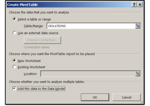
3. In the Create Pivot Defer dialog window, ensure that the Table Range says Violations; the location (choose where to place this report) has the New Worksheet ring box seat curbed; and then check the last box: Add this data to the Information Model; and click OK.

Note: The reason we selected the Violations table instead of the Master or Addresses table is because we want to analyze and calculate the information in this table.

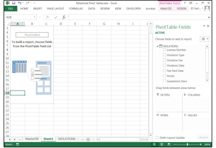
4. The PivotTable Fields panel opens happening the right.

JD Sartain / PC Populace

The PivotTable Fields panel opens on the right when you're working in this mode.

5. Next, select Data > Relationships, and the Manage Relationships duologue window opens. Click the New release on the right, and the Create Relationship window opens.

6. Click the land arrow beside the Table battlefield and select Master1 from the list. In the Column (Foreign) Input boxwood, click the pointer and select LicenseNumber from the list.

7. In the Related Table Stimulus box seat, choose the Violations table. Low Related Column (Primary), click the pointer again and select LicenseNumber once more from that list.

JD Sartain / PC World-wide

Make up Relationships between the Master1 Table and Violations Board.

8. The Manage Relationships dialog window re-appears. Come home the Newly button on the right and the Create Relationship window opens.

9. Click the downwards arrow beside the Defer field again and choice Master1 from the list. In the Tower (Naturalized) Input boxwood, click the arrow and prize LicenseNumber from the list.

JD Sartain / PC World

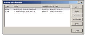
The Manage Relationships window shows two nimble relationships.

10. In the Related Board Input box, select the Addresses postpone. Under Incidental to Column (Firsthand), click the arrow again and choose LicenseNumber again

11. The Manage Relationships dialog window re-appears. Notice that you now stimulate two energetic relationships: Master1 + Violations and Master1 + Addresses. If finished, click O.k. and past Close.

Create the Pivot man Set back reports

1. In the PivotTable W. C. Fields panel, click the wordEntirely at the high.

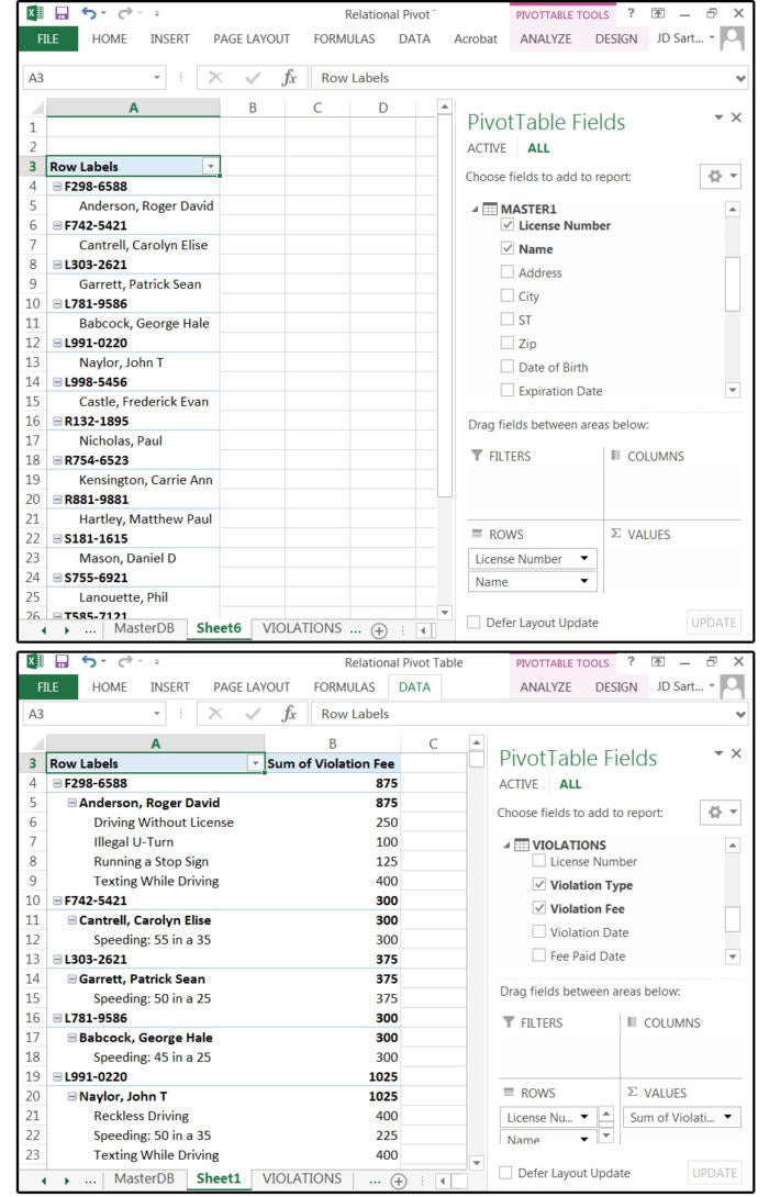
2. Click the Table name pointer to display the W. C. Fields in to each one Postpone. E.g., under the Master1 Table, click the LicenseNumber and Name checkboxes.

3. Under Violations Table, click the Assault Type and Ravishment Fee checkboxes. The PivotTable report appears immediately on the left, flourishing and expanding as you MBD more fields.

JD Sartain / PC Earthly concern

Select fields from the Master1 Prorogue and fields from the Violations table for this paper.

Note: Excel knows which field of view is the key field of view, because you defined the relations using the Pivot Put of tools in the Create Relationship dialog window. So IT's unnecessary to let in the key field (LicenseNumber) in both Tables. If you do, this study will appear twice (in ii different areas) in your report. Unless you need it twice in your describe, don't click this field twice. Once in the Master1 table is enough.

Opine that now your boss wants to see if thither is a connective 'tween the violations and the areas (ZIP Codes) where the offending drivers live. You can Doctor of Osteopathy this well.

4. First, you must ensure that your Travel rapidly Codes are entered as Text fields. Access the Master1 spreadsheet table and play up the Travel rapidly field.

5. Pick out Home > Format> Format cells. Under the Number tab, pick out Text from the list.

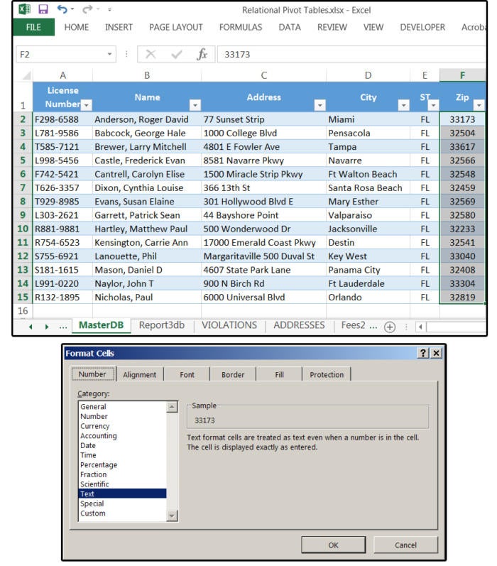JD Sartain / PC World

Ensure your ZIP Code field is defined as a Text field.

6. Scroll endorse to the Master1 Table and click the checkbox beside the field Energy.

7. A yellow box appears within your Pivot Table Fields panel that says: Relationships betwixt Tables may glucinium needed, followed by a Create button. If you click this button and re-delimitate the relationships in the Create Relationship duologue windowpane, Excel displays a message that says: A human relationship already exists between these deuce columns. So click Cancel. Save clock and just click the 'X' in the upper niche to close the yellow loge.

8. If Excel still treats your ZIP arsenic a number and places it into a Aggregate column, right-click the Zip field and choose Move to Rowing Labels from the drop-down menu inclination, Oregon go down to the Values box (bottom right of the Pivot Put over Fields panel), click the arrow, and choose Move to Row Labels from the popup menu list. And the ZIP Codes move infra each violation. Much improved.

JD Sartain / PC Macrocosm

Close the yellow box, then change ZIP Code to Row Labels.

Next, we'll add some more fields to enhance our report.

9. Suction stop the Violation Day of the month checkbox under the Violations Table in the Pin Table William Claude Dukenfield panel. Note that Surpass adds the dates to columns ordinal, which doesn't mould at all. The information is whol o'er the place and too corneous to learn.

10. Powerful-click the Violations Engagement discipline in the Pivot Table Fields panel (beside the checkbox) and select Go down to Row Labels from the drop-pop menu list. Comment the date stamp is placed under the ZIP code and Violation Type. Note that the eldest number one wood on the listing, Roger David Anderson, has two illegal U-turns, one and only connected Feb 10, 2015, and one on Oct 12, 2017.

11. And last, in the Pin Table Fields panel, dawn the Points airfield under the Violations Table (beside the checkbox).

12. Excel adds the field to your report and sums the points away License Number (past driver) and and then as wel adds a Fantastic Total for wholly the Points. Notice how easy IT is to ADHD or murder fields to your reports using the Pivot Table tools.

Promissory note: The subtotals and totals are in bold, and the violations are in regular type. For good example, the data on Roger David Anderson's two black-market U-turns are in regular type, patc the U-turns' subtotal of $100 and 6 points is in boldface.

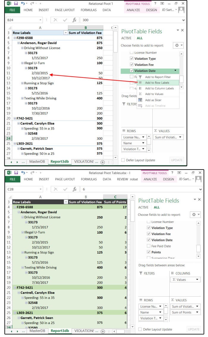JD Sartain / PC World

08 Add two more fields to your reputation: Violation Particular date and Points

Use the Pivot Table Tools / Blueprint tab (only panoptical when the report is active) to add color and creative data format to the Hold over layout. Tables are easier to read when the rows are alternating colours and the field totals are in bold. Experiment and have fun.

Pivot Table Tips

1. Assure that you e'er have more than one spreadsheet in your workbook that's connected/related to incomparable other spreadsheet through with a common, alone field—such as LicenseNumber for our try out.

2. Second, ensure that the Professional table has just ONE LicenseNumber per record, which can then connect to several Slave tables that have multiple LicenseNumber records. This is called a one-to-many an relationship.

3. Ensure that you have selected and defined all the spreadsheets in your workbook as Tables and given them each unique name calling.

4. When stage setting up and defining relationships between tables, the field of operations formats for some of the agnatic tables moldiness be the same. For example, date formats must match—you force out't mix '12/25/2018′ and 'Dec 25, 2018.'

Source: https://www.pcworld.com/article/407669/create-excel-reports-from-multiple-spreadsheets-with-multi-file-pivot-tables.html

Posted by: bennetttommand.blogspot.com

Share this post